Webstory 1: Developing DA of Total Surface Current Velocity data
WS-1: Developing assimilation of TSCV data:
Idealised observation experiments and estimation of velocity forecast error covariances
Jennifer Waters, Matthew Martin, Isabelle Mirouze and Elisabeth Remy
April 2021
1. Introduction
The ocean total surface current velocity (TSCV) is the Lagrangian mean velocity at the instantaneous sea surface (Marié et al., 2020). Accurate forecasting of the ocean TSCV is important for applications such as search and rescue, tracking marine plastic and for coupled ocean/atmosphere/sea-ice/wave forecasting. Direct measurements of the TSCV are currently not available with global coverage. Various satellite missions are being proposed to measure TSCV globally such as SKIM (Ardhuin et al., 2019) and WaCM (Rodriguez et al., 2019). These satellite missions should provide new opportunities for assimilation of velocities into global forecasting systems in the future.
The ESA Assimilation of TSCV (A-TSCV) project aims to investigate the design, implementation and impact of assimilating synthetic TSCV data in global ocean forecasting systems. The project will use observing system simulation experiments (OSSEs) to test the assimilation methodology and provide feedback on the observation requirements for future satellite missions. Synthetic observations are being generated for all standard data types as well as the new observations expected from SKIM-like satellite missions. Two operational global ocean forecasting systems are being developed to assimilate these data in a set of coordinated OSSEs: the FOAM system run at the Met Office (Blockley et al., 2014) and the Mercator Ocean system (Lellouche et al., 2018).
Here we describe preliminary work to compare results of idealised TSCV observation experiments from the FOAM and MOI systems. We also show results of the estimation of horizontal and vertical forecast error covariance information for horizontal velocities.
2. Idealised Observation Experiments
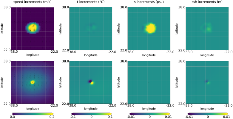
Idealised observation experiments have been performed to demonstrate the increments produced by a single TSCV observation. In both systems TSCV innovations of 0.5 m/s in the zonal and meridional direction are assimilated at the same location. The experiments are configured slightly differently for the two forecast systems due to technical differences. In FOAM only the TSCV observations are assimilated. In the MOI system two experiments are performed with all the standard observations and with and without the TSCV observations, the increments due to the TSCV are calculated from the increment difference between the two experiments. Results for a location in the Mid-Atlantic are presented in Fig 1. The increments for the two systems look very different. The velocity increment is larger for the MOI system and there is a large corresponding sea surface salinity (SSS) increment but very small increments in SSH and temperature. Conversely, there is no SSS increment in FOAM and larger increments in SSH and temperature. The differences in the increments reflects the differences in the forecast error covariance specification and multivariate balance between the two systems.
Figure 1. Surface increments for speed, temperature, salinity and SSH. From MOI (top) and FOAM (bottom).
3. Velocity Error Covariances
FOAM error covariances are prescribed through a set of variances, length-scales and balance relationships. For the assimilation of TSCV data, new variances and length-scales are required for the unbalanced components of zonal (U) and meridional (V) velocities. The velocity balance in NEMOVAR is geostrophic so the unbalanced component represents the ageostrophic velocity component. We have used the NMC method (Parrish and Derber, 1992) to estimate the forecast error covariances. The NMC method used 48 hour and 24 hour forecast difference fields, valid at the same time, as a proxy for the forecast error.
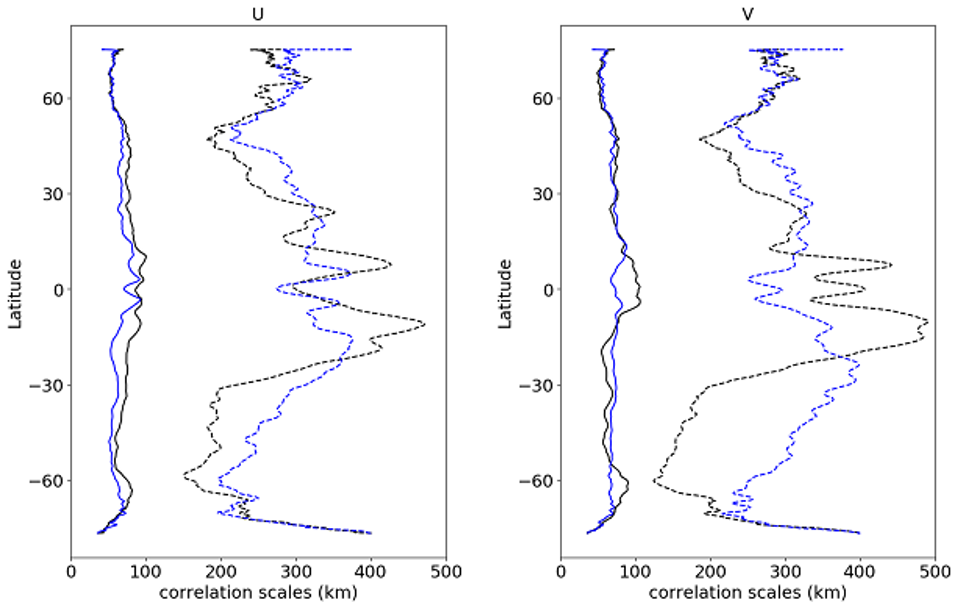
Figure 2. Zonally averaged horizontal forecast error correlation length scales for unbalanced surface U and V. These are estimated by fitting a Gaussian function with two correlation scales to the NMC error covariance data. Black and blue lines are length scales in the x-direction and y-direction, respectively. Dashed and solid lines are the long and short scale, respectively
To produce an estimate of the unbalanced covariances we applied the inverse of the NEMOVAR balance operator to the forecast difference fields to remove the balanced (geostrophic) component. Fig. 2 shows the zonally averaged horizontal background error correlations for September-October-November for U and V. The short scales for U and V vary between around 40km at high latitudes, 70km at mid latitude and 100km in the tropics. The short U length scales have longer scales in the x-direction by 10-20km at most latitudes, while the short V length scales are fairly isotropic expect near the equator. The longer scales vary between approximately 200km in the mid latitudes to 400km near the equator. Long correlations are seen in the x-direction corresponding to the latitude of the North and South equatorial currents. Interestingly the correlations scales are higher in the y-direction in the mid-latitudes which could be due to the boundary currents.
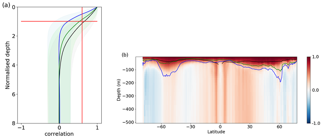
Vertical forecast error correlations for U are shown in Fig. 3 and are compared to an Ekman depth calculated from the model’s vertical eddy viscosity and two mixed layer depth. The MldZ mixed layer depth is defined as the depth at which the density has increased equivalent to a temperature difference of 0.8 degrees at the surface, the MldRho mixed layer depth is the shallowest depth where density increases by 0.01 kgm-3 relative to 10m density. The latitude section plot shows how the correlations vary with latitude. In the profile plot, the global mean error correlations are compared to a normalised depth. When the normalising depth (Ekman depth or Mixed layer depth) is a good approximation to the correlation length scale, the correlation profile passes close to the red line intersect. From Fig. 3, MldZ (which is the mixed layer depth used to parameterise the Temperature and Salinity vertical forecast error correlations in FOAM) significantly over-estimates the U vertical forecast error correlations with the surface, while MldRho and the Ekman depth appear to provide a good approximation to the correlation scales. We plan to test both the MldRho and Ekman depth as a method for parameterising the vertical forecast error correlations in FOAM.
References
Ardhuin F. et al. (2019). SKIM, a Candidate Satellite Mission Exploring Global Ocean Currents and Waves. Frontiers in Marine Science. 6:209. doi: 10.3389/fmars.2019.00209
Blockley, E. W. et al. (2014). Recent development of the Met Office operational ocean forecasting system: an overview and assessment of the new Global FOAM forecasts, Geoscience Model Development, 7, 2613-2638, doi:10.5194/gmd-7-2613-2014.
Marié, L et al (2020). Measuring ocean total surface current velocity with the KuROS and KaRADOC airborne near-nadir Doppler radars: a multi-scale analysis in preparation for the SKIM mission, Ocean Science, 16, 1399–1429, https://doi.org/10.5194/os-16-1399-2020,
Parish, D.F. and Derber, J.C., 1992. The National Meteorological Center’s spectral statistical interpolation analysis system. Monthly Weather Review, 120(8), pp.1747-1763.
Waters, J., Lea, D.J., Martin, M.J., Mirouze, I., Weaver, A. and While, J., 2015. Implementing a variational data assimilation system in an operational ¼ degree global ocean model. Quarterly Journal of the Royal Meteorological Society, 141(687), pp.333-349.
Weaver, A.T., Deltel, C., Machu, E., Ricci, S. and Daget, N. (2005), A multivariate balance operator for variational ocean data assimilation. Quarterly Journal of the Royal Meteorological Society, 131: 3605-3625. doi:10.1256/qj.05.119